R for Basic Statistics - 1

R for Simulation, Sampling and Inference

Simulation

outcomes = c("heads", "tails")

sim_fair_coin = sample(outcomes, prob=c(0.4,0.6) , size=100, replace=TRUE)

barplot(table(sim_fair_coin))

Another use of sample() is to sample n elements randomly from a vector v.

sample(v, n)

To create a vector of size 15 all of whose value are identical:

vector1=rep(0,15)

vector2=rep(NA, 15). NA is often used as placeholder for missing data in R.

For loop in R

for (i in 1:50) {}

Compare to Python (later)

Divide a plot into multiple plots using (following example divides plotting area into three rows and 1 column):

par(mfrow = c(3, 1))

Set the scale of any graph using xlim and ylim arguments.

range() when applied on vector gives a vector of length 2 showing the smallest and largest element of that vector. It is useful to set the scale of graphs using xlim and ylim. For example:

# Define the limits for the x-axis:

xlimits = range(sample_means10)

# Draw the histogram:

hist(sample_means10, breaks=20, xlim=xlimits)

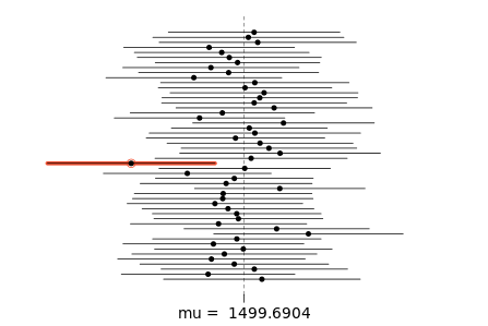
A complete confidence-interval example (comment code later):

# Initialize 'samp_mean', 'samp_sd' and 'n':

samp_mean = rep(NA, 50)

samp_sd = rep(NA, 50)

n = 60

for (i in 1:50) {

   samp = sample(population, n)

   samp_mean[i] = mean(samp)

   samp_sd[i] = sd(samp)

}

# Calculate the interval bounds here:

lower=samp_mean - 1.96*samp_sd/sqrt(n)

upper=samp_mean + 1.96*samp_sd/sqrt(n)

# Plotting the confidence intervals:

pop_mean = mean(population)

plot_ci(lower, upper, pop_mean)

Please note below in the output of the program above, a great use case for plot_ci chart.